• Breadth momentum extends traditional absolute momentum approaches for crash protection.
• Breadth momentum quantifies risk at the universe level by the number of assets with non-positive momentum relative to a breadth protection threshold.
• Vigilant Asset Allocation matches breadth momentum with a responsive momentum filter for targeting offensive annual returns with defensive crash protection.

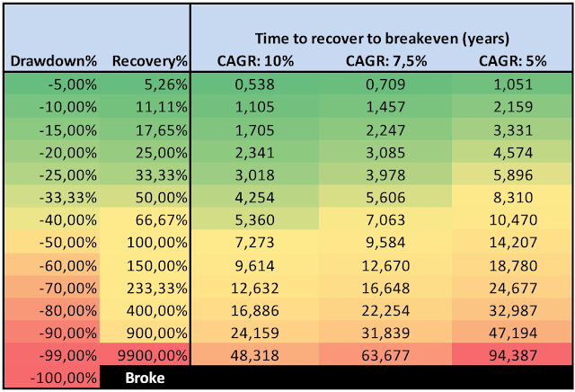
Vigilant Asset Allocation (VAA) is a dual-momentum based investment strategy with a vigorous crash protection and a fast momentum filter. Dual momentum combines absolute (trend following) and relative (cross-sectional) momentum. Contrary to the traditional dual momentum approaches with crash protection through trend following on the asset level, in VAA risk is quantified at the universe level. For superior protection the VAA cash fraction equals the number of assets with non-positive momentum relative to a breadth protection threshold. The combination of breadth momentum with a responsive filter for measuring dual momentum results in a granular crash indicator that allows for targeting offensive annual returns while offering defensive tail risk protection. The VAA methodology is comprehensively explained in our paper published on SSRN. 



The VAA recipe

1. Given a top selection T and a breadth protection threshold B, for each month:
2. Compute 13612W momentum for each asset
3. Pick the best performing assets in the “risk-on” universe as top T
4. Pick the best asset in the “risk-off” universe as safety asset for “cash”
5. Compute the number of assets with non-positive momentum in the “risk-on” universe (b)
6. Compute b/B and round down to multiples of 1/T as “cash fraction” CF for “easy trading”
7. Replace CF of top T by “cash” asset as selected in step 3

13612W momentum filter

In the dual momentum frame work cross-sectional or relative strength momentum is applied for picking the best performing assets for top selection while absolute momentum is utilized to establish whether or not an asset is an uptrend or downtrend (trend following). Different momentum filters are in vogue, like Antonacci’s 12-month return (RET12) for GEM, Keller’s price relative to its 12-month simple moving average (SMA12) for PAA, or Faber’s averaged momentum over the past 1, 3, 6, and 12 months (13612) for GTAA. For VAA we developed a new momentum filter: a variant of the 13612 filter, but now with an even faster response curve by using the average annualized returns over the past 1, 3, 6, and 12 months (13612W). Our 13612W filter has the following composition:

13612W = ( 12 * p0/p1 + 4 * p0/p3 + 2 * p0/p6 + p0/p12 ) / 19 - 1, where pt equals price p with lag t 

This results in monthly return weights for p0/p1, p1/p2, …, p11/p12 of 19, 7, 7, 3, 3, 3, 1, 1, 1, 1, 1, 1, respectively. Notice that our responsive 13612W filter gives a weight of 40% (19/48) to the return over the most recent month as compared to 8% (RET12), 15% (SMA12), and 18% (13612). The following graphic crystallizes the various weighting schemes for the mentioned momentum filters.


Within the VAA frame work our 13612W filter is applied for both relative and absolute momentum.


Quantifying breadth momentum for defensive crash protection

Expanding on the crash protection routine laid down in our PAA-paper, our breadth protection threshold (B) adds granularity and allows for swift allocation adjustments when trend changes occur. Like for PAA, assets are tested on absolute momentum, but now using the responsive 13612W filter, resulting in a number of assets with positive and non-positive momentum respectively (the so-called “bad” and “good” assets). Thus, absolute momentum is applied for establishing a universe’s breadth momentum. Next, our new breadth protection threshold B is defined as the minimum number of “bad” assets (b) for which the strategy is 100% invested in a “risk-off” asset (“cash”). For an N-sized “risk-on” universe, a portfolio’s cash fraction (CF) is determined by the ratio b/B. In formula:

CF=b/B with 0<=CF<=1 limits, where b=0,1,..,N and B<=N.

For more explanation please refer to our paper, or post a question in the comment section.


Easy trading

In the traditional dual momentum approaches (only) top assets are tested on absolute momentum and as a result, the top asset fractions equal the cash fractions. Hence every top asset is replaced by an equal share of cash in case it fails to pass absolute momentum testing. This results in “easy trading” with capital sizes of 1/T: every “bad” asset is simply replaced by “cash”.

Like with PAA, the universe based breadth approach for cash protection is prone to awkward capital sizes which leads to more trading for rebalancing open or initiating new positions. To facilitate “easy trading” (ET) for VAA too, the fractions b/B need to be mapped to a multiple of the top asset fractions 1/T, and the corresponding worst asset(s) from the top T are to be replaced by the found cash fraction CF (the worst assets are those with the lowest 13612W momentum in the top T). Rounding down the raw fractions b/B to multiples of 1/T renders the desired result. In general, the formula for CF with ET through rounding becomes:

CF=(1/T) * floor(b*T/B) with 0<=CF<=1 limits

VAA-G4 with T=1/B=1 & Top=2/B=1 compared to GEM

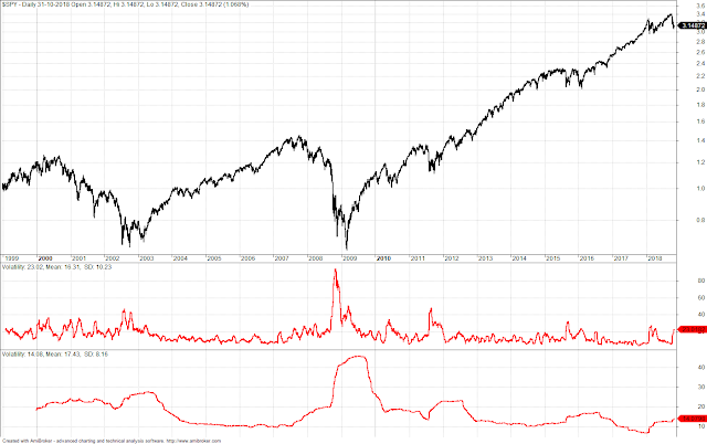
Focusing on concentrated portfolios, the Global 4 (G4) universe from our VAA-paper universes is inspired by Antonacci’s GEM (see post). The ETFs for GEM are VOO (US-stocks) or VEU (global market stocks ex US) and BND (US aggregate bonds) as safety net. To accommodate for sufficient breadth VEU is separated into VEA (developed international market stocks) and VWO (emerging market stocks). Furthermore, BND is added, which leads to an excess return approximation: to be eligible for capital allocation, the stock ETFs have to outperform BND. The “cash” universe is populated with SHY (US short-term treasuries), IEF (US mid-term treasuries), and LQD (US investment grade corporate bonds) to prospect “crisis alpha”.

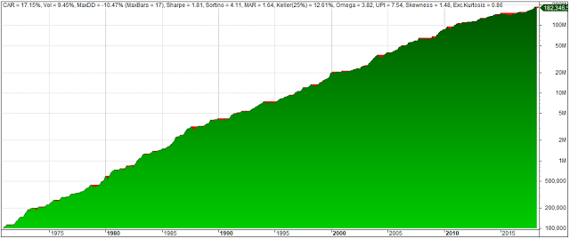
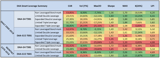
The chart below compares the equity curves and drawdown profiles for two VAA-G4 strategies against GEM over the backtested period: Dec. 1970 – June 2017. VAA-G4 in blue with T=1/B=1 and T=2/B=1 in black. GEM is depicted in red. 

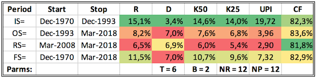
NB! Results are derived from simulated monthly total return data based on indices corrected for tracking errors. Furthermore, trading costs, slippage, and taxes are disregarded. Results are therefore purely hypothetical.

As the above table with the key performance indicators illustrates, both VAA-G4 strategies clearly show outperformance over GEM, not only on “raw” returns, but especially in risk-adjusted terms. Notice the considerable lower drawdowns D and high win-rates for VAA-G4.

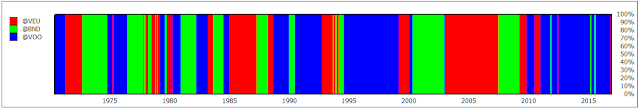
To be fair, the flip-side of VAA-G4’s outperformance (and its responsive 13612W momentum filter) is substantial asset re-allocation as is shown in the following diagrams with VAA-G4 with T=1/B=1 on the upper chart and GEM on the lower one.



Charts for VAA-G4 with T=2/B=1

The following charts provide a detailed view on VAA-G4’s performance with T=2/B=1, being the strategy with the best risk-adjusted performance (see also VAA-paper, note 15).

To summarize: with T=2/B=1, capital is allocated 50:50 into the best two assets out of VOO, VEA, VWO, or BND, provided none of these four assets register non-positive 13612W momentum. However, if any single asset out of these four assets becomes “bad”, all capital is re-allocated to the best asset in the “cash” universe: SHY, IEF, or LQD.

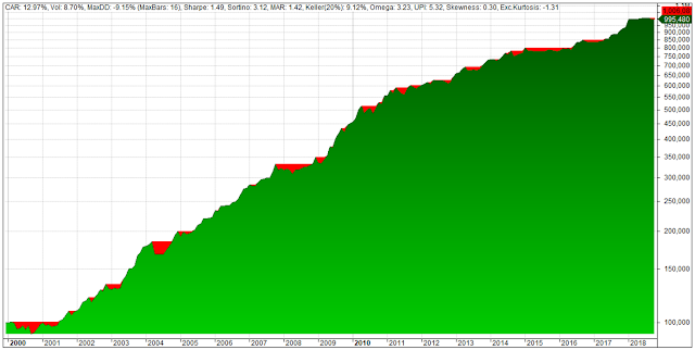
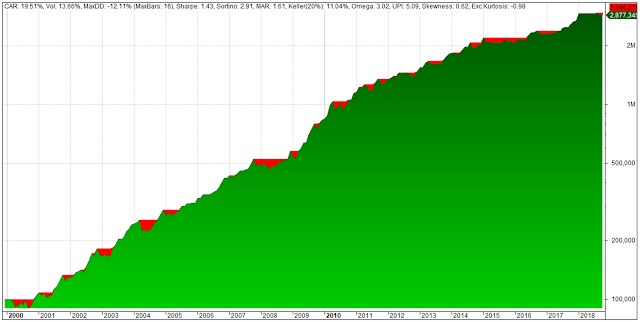
Equity chart with key performance indicators:

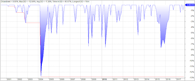
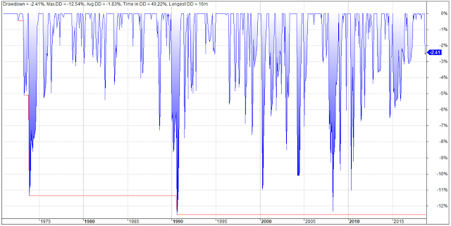
Drawdown chart:

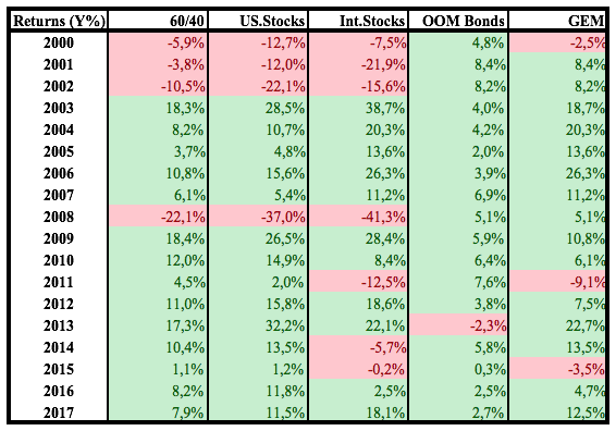
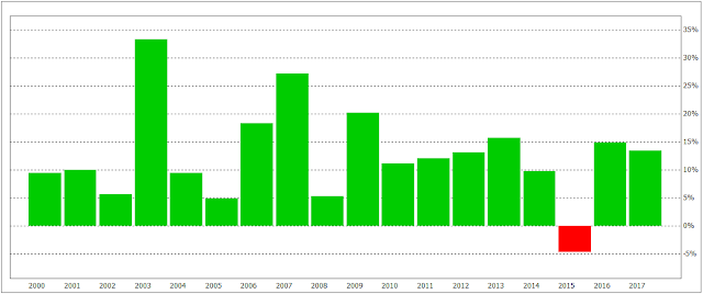
Annual returns:

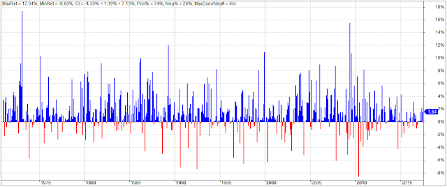
Monthly returns:

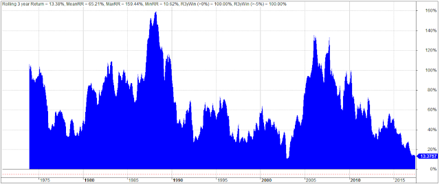
Rolling 3-year returns:

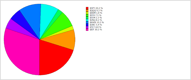
Allocation pie chart:

Profit contribution:

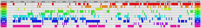
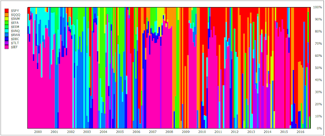
Allocation diagram:


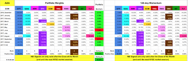
Signal table

[Coming soon]

End notes

• The mentioned GEM, PAA, and GTAA strategies are "real time" monitored by AllocateSmartly.
• The full charts suite for VAA-G4 with T/B=1/1 is available for download (zooming required).
• Investors seeking more diversification might consider VAA-G12 with settings of T=2/B=4, T=3/B=4, T=4/B=4, or T=5/B=5 (see charts suites, zooming required).

The full AmiBroker code for VAA is available upon request. Interested parties are encouraged to support this blog with a donation.

As the new kid on the block, Tiingo is shaking up the data community. Tiingo offers Freemium access to high quality data for an extensive collection covering the full historical record. Starting today historical dividend adjusted data for the Strategy Signals page is sourced from Tiingo's, with delayed current day's NYSE data grabbed "real time"from Google Finance.


For improved performance a dedicated backend caches daily updates from Tiingo's data servers, filters the data into monthly endpoints and operates as on-demand feed for the various Strategy Signal tables.

By popular demand a new beta update is available for the Global Equities Momentum Excel VBA spreadsheet. The new edition sources data from Tiingo's. Following the same work flow as before, the spreadsheet allows to backtest Gary Antonacci's popular GEM strategy (see post).

GEM with mutual funds for longer historical backtest

NB! Backtested results do not reflect actual trading. Furthermore, trading costs, slippage, and taxes are disregarded. Results are therefore purely hypothetical. Terms and conditions apply.

Next to some bug fixes a new pie chart and an annual returns table have been added to the spreadsheet. The pie chart shows the average allocations over the test periode. And the annual returns table specifies GEM's annual returns along with those of the underlying components and the classical 60/40 benchmark.


Tiingo Freemium Account

The new version downloads the ETF/MF data from Tiingo's. Tiingo offers two tailored subscription plans: a free Basic account or a $10/m Power account. A registration/subscription to one of these plans is a prerequisite, because the spreadsheet requires your unique Tiingo token for accessing Tiingo's data server (see instructions in the spreadsheet). To register at Tiingo's: go to Tiingo's welcome page.
NB! After signing up, your personal token is listed on Tiingo's API page (new login required).

Acknowledgements

The current spreadsheet is a modified version of the Excel batch data downloader originally designed by InvestExcel and adapted for GEM by Denis Bergemann. The VBA coding changes related to downloading data from Tiingo, as well as the addition of the allocation pie chart and the annual returns table, were done by William (Will) Johnson, www.Geeks4HireInc.com

Disclaimer

Apart from being a subscriber, no affiliation with Tiingo's at the time of publication.


The Excel sheet for GEM is available upon request. Interested parties are encouraged to support this blog with a donation.

• Adaptive Asset Allocation (AAA) is based on the Nobel Prize winning portfolio theory of Markowitz (1952)
• AAA combines asset’s momentum, volatilities, and cross-correlations for building diversified investment portfolios
• In a tactical application AAA exploits momentum for crash detection and results in consistent returns at mitigated risk levels

Actually, their encounter was coincidental. The fortuitous conversation between a stockbroker and a young mathematician in the early 1950’s proved to be seminal. After the stockbroker learned about the mathematician’s expertise, linear programming and utility maximization, and its real-life applications, he suggested to apply the math to financial portfolios. Fast-forwarding four decades, in 1990 Harry Markowitz shared the Nobel Prize in Economics for his pioneering work on Modern Portfolio Theory (MPT).

Matrix rain animation courtesy TheCodePlayer. AniGif created with Gif Brewery.

The mathematical framework of MPT combines asset’s expected returns, volatilities, and cross-correlations for assembling well-balanced and diversified portfolios while maximizing the expected return for a given level of risk. Its key proposition: for a multi asset portfolio returns can be maximized for a given level of risk. Likewise, risk can be minimized for a desired level of return. With the efficient frontier as its famous graphical depiction (see graph below), Markowitz’ MPT is also known as “mean-variance analysis” since the “mean” or expected return is maximized given a certain level of risk, defined as the portfolio variance (which is volatility squared).


Efficient Frontier

MPT proposes a mathematical framework how investors can reduce overall risk while maximizing return by holding a diversified portfolio of non-correlated asset classes. Instead of looking at the risk-return characteristics of each single asset class, MPT assesses risk and return as cumulative factors for the portfolio as a whole. The Markowitz Efficient Frontier is the graphical depiction of the collection of portfolios that offer the lowest risk for a given level of return. In an excellent video Arif Irfanullah explains in merely 3 minutes how the efficient frontier represents the set of portfolios that will give the highest return at each level of risk or the lowest risk for each level of return (highly recommended).

To illustrate key elements of MPT, let’s bring to bear the top selection from a diversified investment universe SPY, EWJ, VGK, EEM, and DBC (both the full universe population as well as the selection methodology are explained in the next section).

The portfolio concept under consideration for this contribution is the long only minimum variance portfolio without leverage, located at the magenta dot on the outer left side of the purple portfolio cloud (see statistics in bold font in the table below the following graph). For this special case portfolio risk is minimized for all feasible long only combinations. To localize this particular portfolio an Adaptive Asset Allocation (AAA) approach is applied. Please note the purple long only portfolio cloud is only a subset of the full unconstrained long/short portfolio space demarcated by the blue portfolio envelop hyperbola.

Speed readers may jump to the next section, others please bear with me while painting the full picture.


In the above risk-return graph the portfolio space is plotted for every unconstrained long/short portfolio of 5 ETFs: SPY, EWJ, VGK, EEM, and DBC, with portfolio weights summed to 100%. All feasible long/short combinations are contained by the blue portfolio envelop hyperbola, with the efficient frontier being the solid upper boundary and the inefficient frontier the dashed lower one. The grey dots represent 10,000 random unconstrained long/short portfolios. The well-known minimum variance portfolio (MVP) is located at the green cross-mark, being the portfolio with the lowest risk; every single other portfolio combination will result in higher risk. The so-called tangency portfolio (TP) is situated at the red tangent point where the capital allocation line (also in red; basis: 1% risk free rate) touches to the efficient frontier. The TP is suggested to be the mathematical optimal non-leveraged portfolio under the mean variance framework (in the continuation of the video Arif Irfanullah discusses the TP too). On the same capital allocation line, but outside the portfolio envelop, are two particular portfolios depicted. This are two portfolio combinations of the five mentioned ETFs along with a separate risk-free asset: the green dot showing the portfolio with reserved or saved capital and the purple dot the one with borrowed capital (leverage), with target volatilities of 6% and 12%, respectively.

With the long only constraint imposed, each of the orange diamonds depicts a 100% holding in one of the five ETFs, and the purple hurricane shaped cloud represents 5,151 long only portfolios consisting of SPY, EWJ, and DBC (with 1% sized steps). As stated, the long only minimum variance portfolio is to be found at the magenta dot on the outer left side of the purple portfolio cloud. Under the long only constraint, the weights for VGK and EEM are fixed at 0% in order to reach minimal risk (shorting is prohibited). Hence the 3 asset purple portfolio cloud. In the remainder of this contribution the localization and characteristics of this special case portfolio will be assessed.


Adaptive Asset Allocation

As stated, the MPT framework relies on estimates for returns, volatilities, and correlations. Since these estimates are notoriously difficult to predict, especially with regard to the future, a tactical timeframe is adopted for the necessary calculations using a heuristically composed diversified investment universe like the one proposed by the InvestReSolve team (formerly Gestaltu) in their AAA-primer: SPY, VGK, EWJ, EEM, VNQ, RWX, DBC, GLD, TLT, and IEF (see also end notes below).

For starters, each month the best 5 out of 10 ETFs are selected based on their 126-day momentum. Next the minimum variance portfolio is determined as the optimal mix of these five ETFs for obtaining the lowest possible risk (=volatility), using the following steps.

First, for this top half a “weighted” covariance matrix ∑(i,j) is calculated by combining 126-day correlations ρ(i,j) with 20-day volatilities σ(i) and σ(j):

∑(i,j) = ρ(i,j) * σ(i) * σ(j),

where i,j refers to the top 5 ETFs. Finally, the minimum variance portfolio is obtained by minimizing the following matrix formula:

σ² = w'∑w, 

where w is the weights vector with sum equal to 100% and w(i) ≥ 0 and ∑ equals the covariance matrix.

To establish the weight combination that satisfies the minimum variance σ² objective, a Cyclical Coordinate Descent algorithm is deployed (see end notes for sources). For a preset number of cycles, the CCD algo iterates through the weight combinations, approaching closer to the minimum variance objective with each cycle. The following graph demonstrates these iterations going from left to right, minimizing portfolio volatility σ (see the red "helper" dots on the volatility axis too).



Native crash protection

By selecting only the best 5 out of 10 assets, AAA is capable of detecting momentum based trend changes. In up-trending markets capital is allocated into offensive assets, like stocks, REITs, and commodities, while during market sell-offs especially intermediate US-treasuries are in vogue. The following diagram shows the allocation transformations during the bear-bull cycles since the turn of the millennium. Notice the waxing of IEF in periods of market stress (shown for the native InvestResolve universe).


 
Backtesting AAA

The following charts provide a detailed view on AAA’s end-of-month performance using AmiBroker as backtest platform. For this demonstration an alternative investment universe is deployed: SPY, QQQ, IWM, EFA, EEM, VNQ, RWX, DBC, TLT, and IEF.

By substituting VGK, EWJ, and GLD with QQQ, IWM, and EFA the universe at hand is tilted toward domestic US assets, while at the same time demonstrating GLD is not per se required to reach sufficient diversification.

Equity chart with key performance indicators:

NB! Results are derived from simulated daily total return data. Furthermore, trading costs, slippage, and taxes are disregarded. Results are therefore purely hypothetical. Past performance is no guarantee of future results.

Drawdown chart:

Annual returns:

Monthly returns:

Histogram of monthly returns:

Rolling 3-year returns:

Profit contribution:

Average allocation:

Allocation table:

Allocation diagram


Strategy Signals


The signals for the Adaptive Asset Allocation strategy with be available on the Strategy Signals page shortly.


End notes

• The native InvestResolve universe is tracked by AllocateSmartly. Their AAA-post offers additional information along with an extended backtest.
• The AAA-primer by the InvestResolve team and their AAA-book are recommended readings.
• The implementation of the CCD-algorithm as used in the Google Sheet is developed by Roman Rubsamen, a French quant. Modified for AmiBroker, this implementation is also the core element of the AAA-code used for this contribution. On his GitHub repository Roman shares an expanding JavaScript library with portfolio allocation routines.
• Mathematically inclined readers may find the treatise interesting on the CCD algorithm in appendix A.2 of this Smart Beta paper by two other French quants, Jean-Charles Richard and Thierry Roncalli.

The full AmiBroker code for AAA is available upon request. Interested parties are encouraged to support this blog with a donation:

• Many traditional return to risk measures are not apt for intuitive interpretation
• The Keller ratio is expressed as an adjusted return and therefore easy to interpret
• The Keller ratio allows for strategy selection optimally aligned with an investor’s risk appetite

In our VAA-paper we introduced a new metric for assessing a portfolio’s equity line in terms of the reward to risk relationship: return adjusted for drawdown (RAD). We did choose RAD above the usual risk measures like the Sharpe and the MAR ratios (Sharpe: return divided by volatility, MAR: return divided by maximum drawdown), because most retail investors commonly identify true risk with maximum drawdown over volatility. Since RAD is an adjusted return, its interpretation is similar to any return (a simple percentage). For this reason we prefer RAD over MAR, which as such is just a numeric value with little context.

Frankly, albeit return adjusted for drawdown states exactly what RAD is all about, it is quite a mouthful. Therefore, and not only because RAD is his brainchild, but also to commemorate Wouter Keller’s contributions to the TAA literature (FAA, MAA, CAA, EAA, PAA, and VAA; see SSRN) it only seems fitting to accredit the return adjusted for drawdown indicator with his name. So henceforward RAD is to be named the “Keller ratio”.

Celebrating Wouter Keller's 70th birth year

Every investor with skin in the game acknowledges a large portfolio drawdown as the ultimate investing risk. Large drawdowns are devastating to long term returns. For example, during the 2008 subprime crisis the S&P 500 Total Return  index crashed over 50% in approximately 1.5 years from its late 2007 peak, needing 3 years for recovery to breakeven. This left Buy & Hold investors without any positive returns for over nearly five years, not to speak of the excruciating anxiety along the way.

The following table illustrates how severe drawdowns wreak havoc to portfolio performance. Total loss of principal is the biggest risk of all.


Drawdown destroys investment capital, hence the required recovery percentage to get back to breakeven grows exponentially with drawdown. Living through the drawdown quagmire often causes anxiety and can possibly even become a confidence shattering experience. So keeping drawdowns as small as possible is key for ultimate profitability.

As such, maximum drawdown is a “left tail risk”, because it is located in the outer left part of the statistician’s normal distribution chart. In backtests covering only a limited number of years, maximum drawdown may be a single event occurrence. For any meaningful assessment of drawdown long-term backtests are required, preferably extending over multiple decades and comprised of several bull-bear market cycles with many peak-to-trough declines.

The Keller ratio adjusts return for drawdown such as to reflect the severity of the observed maximum drawdown. In case maximum drawdown is small, the return adjustment is only limited. But with large maximum drawdown, the impact of the return adjustment is amplified, in similar fashion to the exponentially growing recovery percentages shown in the above table.

To recall from our VAA-paper, the formula for the Keller ratio (K=RAD) is:

K = R * ( 1 - D / ( 1 - D ) ), if R >= 0% and D <= 50%, and K = 0% otherwise, 

where R = CAGR and D = Maximum Drawdown of the portfolio equity line over the chosen backtest period, with D expressed as a positive value, and for our models measured at month’s ends. This K measure is based on the observation that a maximum drawdown of 50% often leads to the liquidation of a hedge fund. In this case the Keller ratio becomes 0%, independent of CAGR.

The observant reader recognizes the term D / ( 1 - D ) in the Keller formula, which is the algebraic expression of the increase in price necessary for recovery to breakeven at the previous top portfolio capital level after a drawdown of D. At D = 50%, this price gain equals 100%, so the ratio becomes 0%, reflecting the difficulty of getting back to the previous portfolio peak level after a severe drawdown.

Next, by generalizing the Keller formula an adjustable threshold parameter can be implemented at which the Keller ratio becomes 0%. This allows for a tailored Keller measurement for better reflecting an investor’s risk preference:

K( Dmax ) = R * ( 1 - f * D / ( 1 - f * D ) ), 

where f = 0.5 / Dmax, with Dmax being D at which K = 0%.

Accordingly, using 50%, 25%, 20%, and 10% as the respective threshold parameters, the formula for the Keller ratio becomes:

K(50%) = R * ( 1 - D / ( 1 - D ) ), if R >= 0% and D <= 50%, and K(50%) = 0% otherwise.
K(25%) = R * ( 1 - 2D / ( 1 - 2D ) ), if R >= 0% and D <= 25%, and K(25%) = 0% otherwise.
K(20%) = R * ( 1 - 2.5D / ( 1 - 2.5D ) ), if R >= 0% and D <= 20%, and K(20%)  = 0% otherwise.
K(10%) = R * ( 1 - 5D / ( 1 - D ) ), if R >= 0% and D <= 10%, and K(10%)  = 0% otherwise.

The following table crystallizes the effect of the mentioned Keller thresholds for the VAA-G12 strategy covering 1970 - 2017 (mid) as described in our VAA-paper (see also end notes):


NB! Results are derived from simulated monthly total return data. Furthermore, trading costs, slippage, and taxes are disregarded. Results are therefore purely hypothetical. Past performance is no guarantee of future results.

Using the Keller threshold as the allowed maximum portfolio drawdown, the Keller ratio allows the investor to select the strategy scenario optimally aligned with his risk appetite. An investor with an offensive risk profile might still feel comfortable with high drawdowns, therefore using K(50%) as scenario selector resulting in the T1/B4 setting. An investor with a moderate risk tolerance can select K(25%) as threshold value, leading to preference for the T2/B4 setting. With the threshold lowered to K(20%), the preferred scenario leads to a more diversified top T selection with T5/B4. The same T5/B4 scenario is the right choice for the investor with the lowest risk tolerance, as reflected by the K(10%) threshold.

Point to note: with K(20%), by design the indicator value for the T1/B4 scenario becomes 0%, because the registered maximum portfolio drawdown of the T1/B4 scenario (D = 21.13%) exceeds the chosen K(20%) threshold (Dmax = 20%). The same is true for the T1/B4, T2/B4, and T3/B4 scenarios with the K(10%) threshold deployed.

To elaborate our preference for the Keller ratio over the usual ones like the Sharpe and MAR ratio, let’s revisit the reasoning in our VAA-paper. The Sharpe ratio is defined as the annual return R (often in excess over a target return like the risk-free rate) divided by the annual volatility V of the returns. The MAR ratio (similar to the Calmar ratio) is simply annual return R divided by maximum drawdown D (expressed as D >= 0%). Both measures assume that you can apply leverage to arrive at higher R, V and D combinations with the same Sharpe and MAR ratio. But, as we know from leveraged ETFs, this only holds for constant growth (combined with a lending rate equal to the risk-free rate). However, in practice the resulting Sharpe ratio will be much less after leverage. Furthermore, not all investors - especially not retail investors - have access to cheap leverage at (near) risk-free rates. Therefore, when optimizing TAA-models using Sharpe or MAR ratios as target, one might get stuck at relative low returns R with low risk, especially when using a low (near) risk-free or zero target return for the Sharpe threshold.

As an alternative for the Keller ratio the Ulcer Performance Index (UPI) or “Martin Ratio” springs to mind. UPI is return divided by the Ulcer index (UI), where the Ulcer Index measures the depth and duration of percentage drawdowns in price from earlier highs. The greater a drawdown in value, and the longer it takes to recover to earlier highs, the higher the UI. Technically, UI is the square root of the mean of the squared percentage drawdowns in value. The squaring effect penalizes large drawdowns proportionately more than small drawdowns. (From Peter G. Martin’s explanation at tangotools.com). UPI takes the entire drawdown record into account, which is statistically preferable. However, using UPI as target frequently results in lower optimal returns and broad top selections, because in general those diversified tops coincide with smaller drawdowns.

In our current research the Keller ratio is preferred, especially because of its risk targeting through lowering or heightening of the drawdown threshold. However, without the multi decade In-Sample optimization / Out-of-Sample (IS/OS) validation approach, as adhered to in our research, where IS/OS each cover several market cycles, optimizing for the Keller ratio bears the risk of data snooping because maximum drawdown is just a single data point, prone to overfitting.

End notes

• The VAA-strategy is explained is this post: Breadth Momentum and Vigilant Asset Allocation.
• AllocateSmartly will begin tracking VAA-G12 T2/B4 "in the near future".
• Detailed views at the performance of VAA-G12 for the T2/B4, T3/B4, T4/B4, and T5/B4 scenarios are available in the charts suites (zooming required).
• The signals for VAA-G12 with T2/B4 and T5/B4 are available on the Strategy Signals page (with T4/B4 being discontinued shortly).
• This post is currently under review for publication on SeekingAlpha too.

• Defensive Asset Allocation (DAA) builds on the framework designed for Vigilant Asset Allocation (VAA)
• For DAA the need for crash protection is quantified using a separate “canary” universe instead of the full investment universe as with VAA
• DAA leads to lower out-of-market allocations and hence improves the tracking error due to higher in-the-market-rates

In our brand new SSRN-paper “Breadth Momentum and the Canary Universe: Defensive Asset Allocation (DAA)” we improve on our Vigilant Asset Allocation (VAA, see post) by the introduction of a separate “canary” universe for signaling the need for crash protection, using the concept of breadth momentum (see VAA). This protective universe functions as an early warning system similar to the canary in the coal mine back in the day. For DAA the amount of cash is governed by the number of canary assets with negative momentum. The risky part is still based on relative momentum, just like VAA. The resulting investment strategy is called Defensive Assets Allocation (DAA). The aim of DAA is to lower the average cash (or bond) fraction while keeping nearly the same degree of crash protection as with VAA.

Using a very simple model from 1925 to 1970 with only the S&P 500 total return index as investment asset, we arrive at a two-asset canary universe (VWO and BND) combined with a protective B2 breadth momentum setting, which defines DAA’s core elements.

The DAA concept turns out to be quite effective for nearly all four universes examined in our VAA-paper from 1971 to 2018. The average cash fraction of DAA is often less than half that of VAA’s (below 30% instead of nearly 60%), while return and risk are similar and for recent years even better. Deploying a separate “canary” universe for signaling the need for crash protection also improves the tracking error with respect to the passive (buy-and-hold) benchmark due to higher in-the-market-rates than with VAA. The separate “canary” universe also limits turnover. This makes DAA less sensitive for rising cash (or bond) yields, which is key in view of recent low rates.

To crystallize the DAA concept:

1. When both canary assets VWO and BND register negative 13612W momentum, invest 100% in the single best bond of the cash universe;
2. When only one of the canary assets VWO or BND registers negative momentum, allocate 50% in the top half of the best risky assets, while applying equal weights, and invest the remaining 50% in the best bond of the cash universe;
3. When none of canary assets VWO and BND register negative momentum, indicating the risk of a crash is deemed low, invest 100% in the full top risky assets, again applying equal weights. 

As a first demonstration the performance metrics of DAA-G12 are presented in the table below along with the 1971-2018 equity chart. Notice the key performance indicators in the chart’s title. The demonstrated setup consists of 12 global risky assets (G12): SPY, IWM, QQQ, VGK, EWJ, VWO, VNQ, GSG, GLD, TLT, HYG, and LQD. For out-of-market allocation a three asset cash proxy universe is used: SHY, IEF, and LQD. The (fixed) protection universe for quantifying breadth momentum is populated with (only) the mentioned two “canary” assets: VWO and BND. Using DAA’s protective B2 breadth momentum setting, a one dimensional optimization sweep over a top size T of 1, 2, 3, 4, 5, or 6 assets on the IS 1971-1993 period with K(25%) as target, results in T=6 as being the optimal top size for DAA-G12.

NB! Results are derived from simulated monthly total return ETF data. Furthermore, trading costs, slippage, and taxes are disregarded. Results are therefore purely hypothetical. Past performance is no guarantee of future results.

A (nearly) “live” signals table for the Defensive Asset Allocation strategy with the above mentioned setup will be added to the Strategy Signals page in due time. Until then, the table is fully functional below. Please take note of the limitations as mentioned on the Strategy Signals page.

NB! No guarantee whatsoever is given for the soundness of the strategy nor the proper functioning of the table nor for the accuracy of the (time delayed) signals. Please do your own due diligence and use at your peril. The Important Notice in the footer applies as well as the Disclaimer.

The full AmiBroker code for DAA is available upon request. Interested parties are encouraged to support this blog with a donation:

• The constant leverage myth is busted: there is no spoon natural decay. 
• DAA’s fast protective momentum approach successfully detects lower volatility regimes with higher streak potential. 
• Smart leverage through a clever separation of signals and trades can achieve considerable outperformance even on a risk adjusted basis.

Popular belief that constant leveraging results in decay over time is a myth. Michael Gayed and Charles Bilello busted the myth in their 2016 Dow Award winning paper “Leverage for the Long Run”. Their research shows that daily re-leveraging is not without risk. At times the act of re-leveraging can even be mathematically destructive. Yet the source of that risk does not come from some inherent form of natural decay. The authors single out high volatility and seesawing action as the (real) enemies of leverage, while low volatility and streaks in performance are its friends.



When the stock market is in an uptrend - positive 13612W momentum for all canary assets - favorable conditions for leveraged stock positions are assumed targeting positive streaks in performance. When the stock market is in a downtrend - negative 13612W momentum for one or more of the canary assets - a rise in volatility is expected and a (relatively) safe Treasury bond position is acquired to avoid the constant leverage trap for stocks.

On top of DAA’s dedicated 13612W protective momentum deployment for detecting favorable conditions for leverage, the smart leverage approach incorporates a clever separation of signals and trades. As proposed by Matthias Koch, a quant from Germany, non-leveraged asset universes are used for signaling momentum based position sizing while universes that hold a limited number of matching leveraged funds are used for actual trading.

With a modified DAA framework to support the required signal-trade separation, we explore smart leverage based on the diversified G12 ETF portfolio as featured in our DAA-paper: SPY, QQQ, IWM, VGK, EWJ, VWO, GSG, GLD, VNQ, HYG, TLT, and LQD. The demonstration is introduced with the DAA setup as benchmark for the subsequent smart leverage setups.

For readers unfamiliar with the concepts of breadth momentum and protective momentum, the VAA and DAA posts (see here and here) are required reading as these concepts along with the used abbreviations are considered prior knowledge.

Warning: Caution is warranted as leverage involves higher risks to costs and loss.


Volatility regimes

The below daily chart for SPY paints a clear picture with respect to the volatility regimes over the last nearly 20 years. The two sub panes show the annualized volatilities measured over the rolling 21-days (1-month) and 252-days (1-year) respectively. Notice the rise in volatility during bear markets and the drop to lower volatility typical for periods when bull markets are picking up steam. Smart leverage targets those lower volatility regimes because of their higher streak potential.


The accompanying table with SPY’s key performance indicators offers insight into the regime characteristics for the 2000-2018 time frame. Notice the changes in CAR’s and volatilities. To match the above daily chart, the table metrics are obtained with daily endpoints for higher granularity too.


NB! Tables in the remainder of this article are based on monthly endpoints for comparison with previous posts, i.e. on EAA, PAA, VAA, and DAA.


Smart Leverage

The smart leverage approach is demonstrated using the DAA framework. To recall, DAA’s key elements are its fast 13612W momentum filter combined with a dedicated protection universe with only two “canary” assets (VWO and BND) whose absolute momentum readings are decisive for capital allocation between “risky”and “safety” assets.

Smart leverage incorporates a clever separation of signals and trades. Absolute and relative momentum based position sizing is derived from non-leveraged ETF universes, while the actual trading universes may hold matching leveraged ETFs (in bold below).

To crystalize the concept for the DAA smart leverage framework:
Protection: VWO, BND
Signals: SPY,QQQ,IWM,VGK,EWJ,VWO,GSG,GLD,VNQ,HYG, LQD,TLT + SHY,IEF
Trades: SSO,QLD,UWM,VGK,EWJ,VWO,GSG,GLD,URE,HYG,LQD,UBT + SHY,UST


Data

For the portfolio ETFs the daily (leveraged) histories are synthetically extended going back to December 31, 1998. For our favorite setup a long-term backtest is shown too, covering smart leverage over 1971-2018. The long-term backtests are based on monthly data going back to December 31, 1969. Both series use October 31, 2018 as end dates. For both the daily and monthly data based series results are reported by using monthly endpoints for comparison reasons.


Backtests Summary

For both the G4 as well as the G12 universe a comprehensive series of backtests gave the following results. The Appendix holds the used universe compositions along with detailed performance results. The Appendix also shows the benefit of using separate universes for signals and trades.


For the remainder of this post DAA-G12 combined with a limited number of double leveraged assets will be in the spotlights. This is the setup with the highest risk adjusted performance as measured by both K(20%) and UPI from the full series (see last table row).

DAA-G12: The Non-Leveraged Benchmark

The setups for analyzing the global diversified 12 asset portfolio, adhere to DAA’s novel protective momentum approach as introduced in our DAA paper with (always and only) VWO and BND as canary assets. All non-leveraged and leveraged variations use a T6B1 scenario. With a T6 top size rotation, maximum diversification is reached within the top half of the risky R12 universe during lower volatility regimes with higher streak potential. Additionally, with a binary B1 setting DAA reallocates all capital to the best performing safety (treasury) asset in case one or both canary assets register negative 13612W momentum. Only when both VWO and BND register positive 13612W momentum (and only then), risky assets are under consideration for capital allocation. So the used B1 setting keeps defenses high which is key when leveraged assets are involved.

Actually the benchmark setup is quite similar to the setup used in the DAA paper, with the exception of a smaller, treasury only, bond universe: SHY and IEF. Furthermore, since no leverage is involved for the benchmark setup, signal-trade discrimination is superfluous at this point, hence the benchmark signals are derived from the trade universe.

DAA-G12 T6B1 R12 C2 P2 (VWO,BND)
Signals: SPY,QQQ,IWM,VGK,EWJ,VWO,GSG,GLD,VNQ,HYG,TLT,LQD + C2:SHY,IEF
Trades: SPY,QQQ,IWM,VGK,EWJ,VWO,GSG,GLD,VNQ,HYG,TLT,LQD + C2:SHY,IEF


For maximum insight the table shows key performance indicators for 8 distinctive periods with changing market regimes. Our DAA-G12 benchmark achieves both volatility and maximum drawdown readings well below a conservative level of 15%, hence the use of the Keller ratio with a (low) 20% threshold (for more on the Keller ratio see here).


DAA-G12: Limited Double Leverage 

Next the proposed signal-trade separation is deployed for analyzing smart leverage with mixed leveraged and non-leveraged trade universes. Adding double leverage assets, for the R12 portfolio SPY, QQQ, IWM, VNQ, and TLT are replaced by SSO, QLD, UWM, URE, and UBT respectively, while IEF is exchanged for UST on the bonds side. Furthermore signal-trade separation is deployed to ascertain the discrimination effect of the permanent P2 protection universe. All other settings are kept equal to those of the benchmark setup.

DAA-G12 T6B1 R12 C3 P2 (VWO,BND)
Signals: SPY,QQQ,IWM,VGK,EWJ,VWO,GSG,GLD,VNQ,HYG, LQD,TLT + C2:SHY,IEF
Trades: SSO,QLD,UWM,VGK,EWJ,VWO,GSG,GLD,URE,HYG,LQD,UBT + C2:SHY,UST


Referencing the benchmark, the smart leverage setup achieves considerable higher CAR metrics but at the cost of higher volatilities and worse maximum drawdowns. The better K(20%) readings for all but one sub period combined with mostly somewhat lower but still impressive UPI readings demonstrate the robustness of the smart leverage approach on a risk adjusted basis.

A comparison of the following table with the previous one displays the benefit of using separate signal and trade universes for the DAA-G12 setup with its dedicated P2 protection universe. Omitting the separation between signals and trades results in deteriorated performance on both a raw return and a risk adjusted basis for a multitude of metrics on most sub periods.

Signals: SSO,QLD,UWM,VGK,EWJ,VWO,GSG,GLD,URE,HYG,LQD,UBT + C2:SHY,UST
Trades: SSO,QLD,UWM,VGK,EWJ,VWO,GSG,GLD,URE,HYG,LQD,UBT + C2:SHY,UST



Long-term Impression: DAA-G12 with Limited Double Leverage

A long-term monthly look from December 31, 1970 (excluding 13612W’s initialization period of 1-year) until October 31, 2018 at the global diversified portfolio concludes the demonstration of the smart leverage approach. The used setup has again a T6B1 rotation scenario for maximum diversification within the G12 portfolio’s top half. The protective B1 setting makes sure that the portfolio rotates 100% into safe treasury assets at the first sign of weakness within the canary assets as measured by their 13612W momentum.

For the above series of comparisons ETFs were used with synthetically extended daily (leveraged) histories going back to December 31, 1998. Since daily index data going back as far as December 31, 1969 is hard to find, if even available, the below used long-term approximations of leveraged assets are derived from monthly total return data (so with monthly instead of daily resets). Therefore the results of the following backtests are merely an impression how the smart leverage approach might have performed over the last nearly 50 years.

In familiar fashion first the equity chart of the non-leveraged benchmark portfolio is shown, followed again by the chart of the limited double leveraged portfolio.

DAA-G12 T6B1 R12 C2 P2 (VWO,BND)
Signals: SPY,QQQ,IWM,VGK,EWJ,VWO,GSG,GLD,VNQ,HYG, LQD,TLT + C2:SHY,IEF
Trades: SPY,QQQ,IWM,VGK,EWJ,VWO,GSG,GLD,VNQ,HYG, LQD,TLT + C2:SHY,IEF


For the benchmark setup the impact of the 1970s “Oil Shock” is visible in the chart, but due to the highly diversified T6 top size the shock effect is mitigated to a great extent. Furthermore the benchmark using only non-leveraged assets shows impressive performance metrics with an overall CAR of 16.50% combined with very low volatility (8.36%) and maximum drawdown (-8.00%) readings. As a result the overall risk adjusted metrics are nothing less than outstanding.

Next up is the smart leverage setup with its typical signal-trade separation combined with limited double leveraged universes.

DAA-G12 T6B1 R12 C2 P2 (VWO,BND)
Signals: SPY,QQQ,IWM,VGK,EWJ,VWO,GSG,GLD,VNQ,HYG, LQD,TLT + C2:SHY,IEF
Trades: SSO,QLD,UWM,VGK,EWJ,VWO,GSG,GLD,URE,HYG,LQD,UBT + C2:SHY,UST


Referencing the benchmark, over the backtested period of nearly half a century the smart leverage setup achieves a nearly 50% higher CAR reading of 23.78% against 16.50% for the non-leveraged setup. Volatility and maximum drawdown increase by roughly the same ratio. Noteworthy, the maximum drawdown level of 12.54% is still well contained below our 15% mark. The risk adjusted K(20%) metric of the smart leverage setup even beats the one of the benchmark and MAR and UPI readings are only slightly lower. Again, this demonstrates the robustness of the smart leverage approach both on a raw return basis as well as on a risk adjusted basis.


Long-term Charts

To conclude our exploration of smart leverage with the the DAA-G12 approach with its protective momentum through dedicated canary assets and signal-trade separation, a couple of extra charts are shown to allow for a detailed impression of its long-term performance.

Annual returns:

Monthly maximum drawdowns:

Profit contribution:

Monthly returns and win-rates:
  
Rolling 1-year returns:


Conclusion

Smart leverage with the demonstrated DAA-G12 setup using signal-trade separation manages to steer clear from the constant leverage trap. Combining smart leverage's clever separation of signals and trades together with DAA's novel canary protection proves successful in detecting lower volatility regimes and banks on its higher streak potential resulting in considerable outperformance for both raw and risk adjusted returns as measured with the conservative K(20%) ratio.


Endnotes and cautions

• All reported results are derived from simulated total return ETF data. Furthermore, trading costs, slippage, and taxes are disregarded. Results are therefore purely hypothetical and no investor could have attained these results. The presented results are no guarantee of future returns. Especially for synthesizing extended data series of leveraged ETFs expense ratios along with the the impact of historically higher borrowing costs are difficult to estimate.
• Liquidity, low trading volumes, and assets-under-management requirements limit the practical application of leveraged assets to avoid high slippage costs. These limitations may cause to be problematic in times of market stress when spreads typically widen. Caveat emptor!
• Contrary to the mainly decreasing interest rates environment during the analyzed period, the regime for foreseeable future may be characterized by rising rates. Most likely this will have a negative impact on the reported results.
• Recommended further reading: “Trend Following on Steroids” by Wouter Keller and our forthcoming paper on DAA combined with smart leverage. Furthermore we have included a smart leverage example in the latest update of our DAA-paper on SSRN (see section 9).

The full AmiBroker code for DAA's Smart Leverage framework is available upon request. Interested parties are encouraged to support this blog with a donation:

Due to a change in the placement of OHLC price data in Tiingo's feed, the spreadsheet should no longer be used! 

A revision is currently under construction.

Hybrid Asset Allocation (HAA) is a novel approach which combines “traditional” dual momentum with “canary” momentum. Dual momentum is based on the concept of assets price trends and consists of absolute (trend following) and relative (cross-sectional) momentum. In addition to the traditional dual momentum framework HAA adds an extra layer for crash protection at the portfolio level based on a single canary asset in the protective (or canary) universe. HAA allows only for offensive investments when the canary asset is uptrending and switches in full to defensive investments if and for as long as this asset is not uptrending. Interested readers are referred to our paper published on SSRN which offers a comprehensive explanation of the HAA methodology including explanations of the used jargon and abbreviations.

Disclosure: as an experiment AI rendered the above text—more or less.